39 add data labels to excel chart
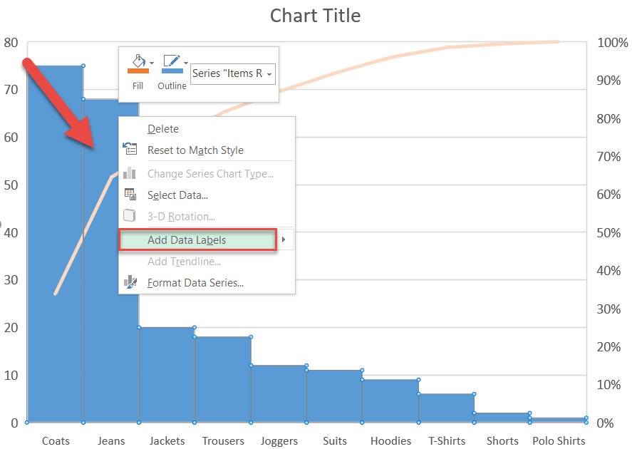
How to add data labels from different column in an Excel chart? This method will introduce a solution to add all data labels from a different column in an Excel chart at the same time. Please do as follows: 1. Right click the data series in the chart, and select Add Data Labels > Add Data Labels from the context menu to add data labels. 2. Add or remove data labels in a chart - support.microsoft.com Add data labels to a chart Click the data series or chart. To label one data point, after clicking the series, click that data point. In the upper right corner, next to the chart, click Add Chart Element > Data Labels. To change the location, click the arrow, and choose an option.
How to Add Axis Labels in Excel Charts - Step-by-Step (2022) How to Add Axis Labels in Excel Charts – Step-by-Step (2022) An axis label briefly explains the meaning of the chart axis. It’s basically a title for the axis. Like most things in Excel, it’s super easy to add axis labels, when you know how. So, let me show you 💡. If you want to tag along, download my sample data workbook here.

Add data labels to excel chart
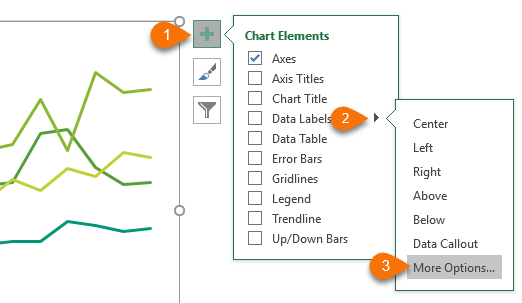
Change the format of data labels in a chart To get there, after adding your data labels, select the data label to format, and then click Chart Elements > Data Labels > More Options. To go to the appropriate area, click one of the four icons ( Fill & Line, Effects, Size & Properties ( Layout & Properties in Outlook or Word), or Label Options) shown here. The XY Chart Labeler Add-in - AppsPro Jul 01, 2007 · The XY Chart Labeler. A very commonly requested Excel feature is the ability to add labels to XY chart data points. The XY Chart Labeler adds this feature to Excel. The XY Chart Labeler provides the following options: Add XY Chart Labels - Adds labels to the points on your XY Chart data series based on any range of cells in the workbook. Add a Horizontal Line to an Excel Chart - Peltier Tech Sep 11, 2018 · Copy the data, select the chart, and Paste Special to add the data as a new series. Right click on the added series, and change its chart type to XY Scatter With Straight Lines And Markers (again, the markers are temporary).
Add data labels to excel chart. How to Make a Pie Chart in Excel & Add Rich Data Labels to The Chart! Sep 08, 2022 · A pie chart is used to showcase parts of a whole or the proportions of a whole. There should be about five pieces in a pie chart if there are too many slices, then it’s best to use another type of chart or a pie of pie chart in order to showcase the data better. In this article, we are going to see a detailed description of how to make a pie chart in excel. Edit titles or data labels in a chart - support.microsoft.com To reposition all data labels for an entire data series, click a data label once to select the data series. To reposition a specific data label, click that data label twice to select it. This displays the Chart Tools , adding the Design , Layout , and Format tabs. How to Add Total Data Labels to the Excel Stacked Bar Chart Apr 03, 2013 · Step 4: Right click your new line chart and select “Add Data Labels” Step 5: Right click your new data labels and format them so that their label position is “Above”; also make the labels bold and increase the font size. Step 6: Right click the line, select “Format Data Series”; in the Line Color menu, select “No line” How to add data labels in excel to graph or chart (Step-by-Step) Add data labels to a chart. 1. Select a data series or a graph. After picking the series, click the data point you want to label. 2. Click Add Chart Element Chart Elements button > Data Labels in the upper right corner, close to the chart. 3. Click the arrow and select an option to modify the location. 4.
How to create Custom Data Labels in Excel Charts - Efficiency 365 Create the chart as usual. Add default data labels. Click on each unwanted label (using slow double click) and delete it. Select each item where you want the custom label one at a time. Press F2 to move focus to the Formula editing box. Type the equal to sign. Now click on the cell which contains the appropriate label. How to Use Cell Values for Excel Chart Labels - How-To Geek Mar 12, 2020 · Select the chart, choose the “Chart Elements” option, click the “Data Labels” arrow, and then “More Options.” Uncheck the “Value” box and check the “Value From Cells” box. Select cells C2:C6 to use for the data label range and then click the “OK” button. How to Make a Gantt Chart in PowerPoint (6 Steps) | ClickUp To edit your Gantt chart in PowerPoint, follow these steps: Click the "Format" tab and choose "Chart Tools". Select the drop-down arrow next to "Chart Layouts," then click " Insert Blank Chart". Click on the "Format Axis" button (the one with a horizontal line) and choose an axis type from the menu that appears (e.g., linear ... Data Labels in Excel Pivot Chart (Detailed Analysis) Before adding the Data Labels, we need to create the Pivot Chart in the beginning. We can create a Pivot Chart from the Insert tab. To do this, go to Insert tab > Tables group. Then in the dialog box, select the range of cells of the primary dataset., here the range of cells is B4:J23. And select the New Worksheet in the next option.
How to Insert Axis Labels In An Excel Chart | Excelchat Figure 1 – How to add axis titles in Excel. Add label to the axis in Excel 2016/2013/2010/2007. We can easily add axis labels to the vertical or horizontal area in our chart. The method below works in the same way in all versions of Excel. How to add horizontal axis labels in Excel 2016/2013 . We have a sample chart as shown below; Figure 2 ... Edit titles or data labels in a chart - support.microsoft.com On a chart, click one time or two times on the data label that you want to link to a corresponding worksheet cell. The first click selects the data labels for the whole data series, and the second click selects the individual data label. Right-click the data label, and then click Format Data Label or Format Data Labels. How to Make a Pie Chart in Excel & Add Rich Data Labels to The Chart! Creating and formatting the Pie Chart. 1) Select the data. 2) Go to Insert> Charts> click on the drop-down arrow next to Pie Chart and under 2-D Pie, select the Pie Chart, shown below. 3) Chang the chart title to Breakdown of Errors Made During the Match, by clicking on it and typing the new title. How To Add Data Labels In Excel - danielsadventure.info Click on the arrow next to data labels to change the position of where the labels are in relation to the bar chart. Add A Label (Form Control) Click Developer, Click Insert, And Then Click Label. You can now configure the label as required — select the content of. To format data labels in excel, choose the set of data labels to format.
How to add data labels from different column in an Excel chart?
How to Add Two Data Labels In Excel Chart? - YouTube In this video tutorial, we are going to learn, how to add multiple data labels in excel pie chart.Our YouTube Channels Travel Volg Channelhttps:// ...

How to add live total labels to graphs and charts in Excel ...
Add or remove data labels in a chart - support.microsoft.com Add data labels to a chart Click the data series or chart. To label one data point, after clicking the series, click that data point. In the upper right corner, next to the chart, click Add Chart Element > Data Labels. To change the location, click the arrow, and choose an option.

How to Add Total Data Labels to the Excel Stacked Bar Chart ...
Add or remove data labels in a chart - support.microsoft.com Depending on what you want to highlight on a chart, you can add labels to one series, all the series (the whole chart), or one data point. Add data labels. You can add data labels to show the data point values from the Excel sheet in the chart. This step applies to Word for Mac only: On the View menu, click Print Layout.
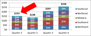
How to Add Totals to Stacked Charts for Readability - Excel ...
How to add a line in Excel graph: average line, benchmark, etc. Right-click the selected data point and pick Add Data Label in the context menu: The label will appear at the end of the line giving more information to your chart viewers: Add a text label for the line. To improve your graph further, you may wish to add a text label to the line to indicate what it actually is. Here are the steps for this set up:

How to add data labels from different column in an Excel chart?
Add a DATA LABEL to ONE POINT on a chart in Excel Click on the chart line to add the data point to. All the data points will be highlighted. Click again on the single point that you want to add a data label to. Right-click and select ' Add data label ' This is the key step! Right-click again on the data point itself (not the label) and select ' Format data label '.
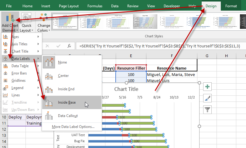
Excel 2016 Gantt Chart Add Data Labels - Excel Dashboard ...
How to add data labels from different column in an Excel chart? Right click the data series in the chart, and select Add Data Labels > Add Data Labels from the context menu to add data labels. 2. Click any data label to select all data labels, and then click the specified data label to select it only in the chart. 3.

How to Use Cell Values for Excel Chart Labels
Lesson 38 - How to add DATA LABELS to charts in Excel Change colour of ... فيديو Lesson 38 - How to add DATA LABELS to charts in Excel Change colour of pie-chart segments in Excel شرح Habib's ICT Tutorials.

Using the CONCAT function to create custom data labels for an ...
How to Add Two Data Labels in Excel Chart (with Easy Steps) Step 4: Format Data Labels to Show Two Data Labels. Here, I will discuss a remarkable feature of Excel charts. You can easily show two parameters in the data label. For instance, you can show the number of units as well as categories in the data label. To do so, Select the data labels. Then right-click your mouse to bring the menu.

how to add data labels into Excel graphs — storytelling with data
How to Add Data Labels in Excel - Excelchat | Excelchat After inserting a chart in Excel 2010 and earlier versions we need to do the followings to add data labels to the chart; Click inside the chart area to display the Chart Tools. Figure 2. Chart Tools Click on Layout tab of the Chart Tools. In Labels group, click on Data Labels and select the position to add labels to the chart. Figure 3.

Is there a way to add data labels as percentages on the ...
How to Add Data Labels to Scatter Plot in Excel (2 Easy Ways) - ExcelDemy Follow the ways we stated below to remove data labels from a Scatter Plot. 1. Using Add Chart Element At first, go to the sheet Chart Elements. Then, select the Scatter Plot already inserted. After that, go to the Chart Design tab. Later, select Add Chart Element > Data Labels > None. This is how we can remove the data labels.
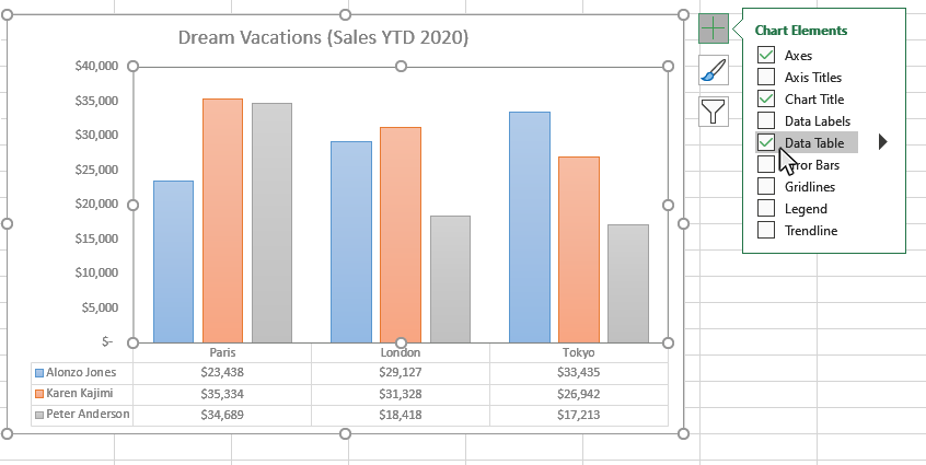
How to Add Data Tables to a Chart in Excel - Business ...
How to add data labels from different column in an Excel chart? Right click the data series in the chart, and select Add Data Labels > Add Data Labels from the context menu to add data labels. 2. Click any data label to select all data labels, and then click the specified data label to select it only in the chart. 3.

Quick Tip: Excel 2013 offers flexible data labels | TechRepublic
Add or remove data labels in a chart Add data labels to a chart Click the data series or chart. To label one data point, after clicking the series, click that data point. In the upper right corner, next to the chart, click Add Chart Element > Data Labels. To change the location, click the arrow, and choose an option.

How to Add Total Data Labels to the Excel Stacked Bar Chart ...
How to add or move data labels in Excel chart? - ExtendOffice To add or move data labels in a chart, you can do as below steps: In Excel 2013 or 2016. 1. Click the chart to show the Chart Elements button . 2. Then click the Chart Elements, and check Data Labels, then you can click the arrow to choose an option about the data labels in the sub menu. See screenshot:
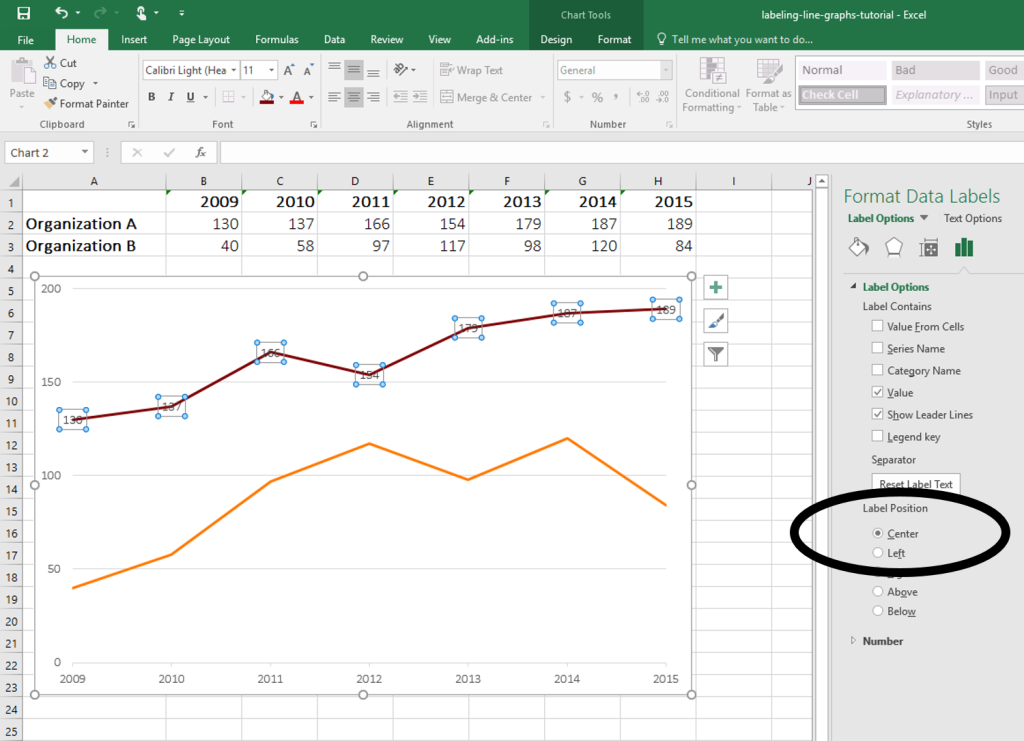
How to Place Labels Directly Through Your Line Graph in ...
Add data labels and callouts to charts in Excel 365 - EasyTweaks.com The steps that I will share in this guide apply to Excel 2021 / 2019 / 2016. Step #1: After generating the chart in Excel, right-click anywhere within the chart and select Add labels . Note that you can also select the very handy option of Adding data Callouts.

microsoft excel - Adding data label only to the last value ...
Add a data series to your chart - support.microsoft.com Right-click the chart, and then choose Select Data. The Select Data Source dialog box appears on the worksheet that contains the source data for the chart. Leaving the dialog box open, click in the worksheet, and then click and drag to select all the data you want to use for the chart, including the new data series.
excel - VBA Pivot Chart data labels not appear - Stack Overflow
Custom Chart Data Labels In Excel With Formulas - How To Excel At Excel Follow the steps below to create the custom data labels. Select the chart label you want to change. In the formula-bar hit = (equals), select the cell reference containing your chart label's data. In this case, the first label is in cell E2. Finally, repeat for all your chart laebls.
Dynamically Label Excel Chart Series Lines • My Online ...
Add a Horizontal Line to an Excel Chart - Peltier Tech Sep 11, 2018 · Copy the data, select the chart, and Paste Special to add the data as a new series. Right click on the added series, and change its chart type to XY Scatter With Straight Lines And Markers (again, the markers are temporary).

Change the format of data labels in a chart
The XY Chart Labeler Add-in - AppsPro Jul 01, 2007 · The XY Chart Labeler. A very commonly requested Excel feature is the ability to add labels to XY chart data points. The XY Chart Labeler adds this feature to Excel. The XY Chart Labeler provides the following options: Add XY Chart Labels - Adds labels to the points on your XY Chart data series based on any range of cells in the workbook.

Solved: How to show all detailed data labels of pie chart ...
Change the format of data labels in a chart To get there, after adding your data labels, select the data label to format, and then click Chart Elements > Data Labels > More Options. To go to the appropriate area, click one of the four icons ( Fill & Line, Effects, Size & Properties ( Layout & Properties in Outlook or Word), or Label Options) shown here.
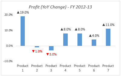
Color Negative Chart Data Labels in Red with downward arrow

How to add live total labels to graphs and charts in Excel ...

Add or remove data labels in a chart

Add data labels and callouts to charts in Excel 365 ...
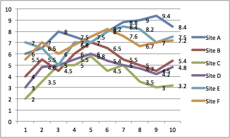
Directly Labeling Excel Charts - PolicyViz

Adding rich data labels to charts in Excel 2013 | Microsoft ...
How to Create a Pareto Chart in Excel – Automate Excel

How to Add Two Data Labels in Excel Chart (with Easy Steps ...

How do I add Data Labels for multiple Low Points Only! : r/excel

Change the format of data labels in a chart

Format Data Labels in Excel- Instructions - TeachUcomp, Inc.

Add or remove data labels in a chart

Improve your X Y Scatter Chart with custom data labels

How to Change Excel Chart Data Labels to Custom Values?

How to Use Cell Values for Excel Chart Labels

Add a Data Callout Label to Charts in Excel 2013 – Software ...

Adding rich data labels to charts in Excel 2013 | Microsoft ...

Add or remove data labels in a chart

How to Add Data Labels in Excel - Excelchat | Excelchat

Change the format of data labels in a chart
Post a Comment for "39 add data labels to excel chart"