40 how to add percentage data labels in excel bar chart

Showing percentages above bars on Excel column graph Update the data labels above the bars to link back directly to other cells Method 2 by step add data-lables right-click the data lable goto the edit bar and type in a refence to a cell (C4 in this example) this changes the data lable from the defulat value (2000) to a linked cell with the 15% Share answered Nov 20, 2013 at 0:30 brettdj How to Add Total Data Labels to the Excel Stacked Bar Chart For stacked bar charts, Excel 2010 allows you to add data labels only to the individual components of the stacked bar chart. The basic chart function does not allow you to add a total data label that accounts for the sum of the individual components. Fortunately, creating these labels manually is a fairly simply process.

How to Display Percentage in an Excel Graph (3 Methods) If you want to change the graph axis format from the numbers to percentages, then follow the steps below: First of all, select the cell ranges. Then go to the Insert tab from the main ribbon. From the Charts group, select any one of the graph samples. Now double click on the chart axis that you want to change to percentage.

How to add percentage data labels in excel bar chart

Show both value and percentage on Waterfall Chart Re: Show both value and percentage on Waterfall Chart. Tim -. For this, add a series to the chart. For X values, use the category labels of the. waterfall data. For Y values, use the value at the top of the visible bar (s) at each. category. Construct the label text in a parallel worksheet range. After adding the series (it'll probably be ... Column Chart That Displays Percentage Change or Variance 2. Create the Column Chart. The first step is to create the column chart: Select the data in columns C:E, including the header row. On the Insert tab choose the Clustered Column Chart from the Column or Bar Chart drop-down. The chart will be inserted on the sheet and should look like the following screenshot. How to show percentages in stacked column chart in Excel? - ExtendOffice Add percentages in stacked column chart 1. Select data range you need and click Insert > Column > Stacked Column. See screenshot: 2. Click at the column and then click Design > Switch Row/Column. 3. In Excel 2007, click Layout > Data Labels > Center . In Excel 2013 or the new version, click Design > Add Chart Element > Data Labels > Center. 4.

How to add percentage data labels in excel bar chart. How can I show percentage change in a clustered bar chart? Double-click it to open the "Format Data Labels" window. Now select "Value From Cells" (see picture below; made on a Mac, but similar on PC). Then point the range to the list of percentages. If you want to have both the value and the percent change in the label, select both Value From Cells and Values. This will create a label like: -12% 1.729.711 How to Show Percentages in Stacked Bar and Column Charts - Excel Tactics How to Show Percentages in Stacked Bar and Column Charts Quick Navigation 1 Building a Stacked Chart 2 Labeling the Stacked Column Chart 3 Fixing the Total Data Labels 4 Adding Percentages to the Stacked Column Chart 5 Adding Percentages Manually 6 Adding Percentages Automatically with an Add-In 7 Download the Stacked Chart Percentages Example File Add Value Label to Pivot Chart Displayed as Percentage If you use the hidden line method: How to Add Total Data Labels to the Excel Stacked Bar Chart and then use the code mentioned in post #2 to create boxes offset from the hidden line points, you should be able to place the additional labels where you want. You must log in or register to reply here. Similar threads E Add data labels and callouts to charts in Excel 365 - EasyTweaks.com Step #1: After generating the chart in Excel, right-click anywhere within the chart and select Add labels . Note that you can also select the very handy option of Adding data Callouts. Step #2: When you select the "Add Labels" option, all the different portions of the chart will automatically take on the corresponding values in the table ...

How to create a chart with both percentage and value in Excel? Select the data range that you want to create a chart but exclude the percentage column, and then click Insert > Insert Column or Bar Chart > 2-D Clustered Column Chart, see screenshot: 2. How to Add Percentage Axis to Chart in Excel To do this, we will select the whole table again, and then go to Insert >> Charts >> 2-D Columns: To show percentages on a second axis, we first need to click anywhere on the orange bars that we have on our graph (this is not easy in this example as they are rather small). Once we do, we will right-click on it, and then select Format Data Series: How to Show Percentages in Stacked Column Chart in Excel? Follow the below steps to show percentages in stacked column chart In Excel: Step 1: Open excel and create a data table as below. Step 2: Select the entire data table. Step 3: To create a column chart in excel for your data table. Go to "Insert" >> "Column or Bar Chart" >> Select Stacked Column Chart. Step 4: Add Data labels to the chart. Count and Percentage in a Column Chart - ListenData Steps to show Values and Percentage 1. Select values placed in range B3:C6 and Insert a 2D Clustered Column Chart (Go to Insert Tab >> Column >> 2D Clustered Column Chart). See the image below Insert 2D Clustered Column Chart 2. In cell E3, type =C3*1.15 and paste the formula down till E6 Insert a formula 3.

How to show data label in "percentage" instead of - Microsoft Community If so, right click one of the sections of the bars (should select that color across bar chart) Select Format Data Labels Select Number in the left column Select Percentage in the popup options In the Format code field set the number of decimal places required and click Add. Change the format of data labels in a chart To get there, after adding your data labels, select the data label to format, and then click Chart Elements > Data Labels > More Options. To go to the appropriate area, click one of the four icons ( Fill & Line, Effects, Size & Properties ( Layout & Properties in Outlook or Word), or Label Options) shown here. HOW TO CREATE A BAR CHART WITH LABELS ABOVE BAR IN EXCEL - simplexCT In the Format Data Labels pane, under Label Options selected, set the Label Position to Inside End. 16. Next, while the labels are still selected, click on Text Options, and then click on the Textbox icon. 17. Uncheck the Wrap text in shape option and set all the Margins to zero. The chart should look like this: 18. Add or remove data labels in a chart - support.microsoft.com Click the data series or chart. To label one data point, after clicking the series, click that data point. In the upper right corner, next to the chart, click Add Chart Element > Data Labels. To change the location, click the arrow, and choose an option. If you want to show your data label inside a text bubble shape, click Data Callout.

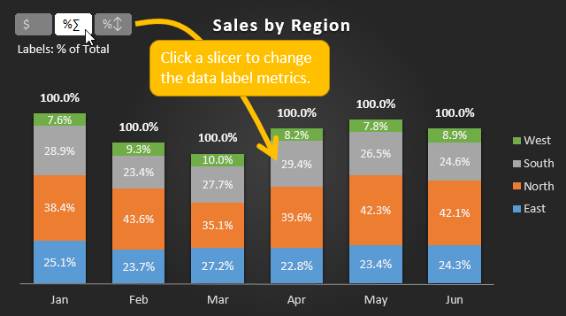
Create Dynamic Chart Data Labels with Slicers - Excel Campus

How to Add Data Labels to an Excel 2010 Chart - dummies Use the following steps to add data labels to series in a chart: Click anywhere on the chart that you want to modify. On the Chart Tools Layout tab, click the Data Labels button in the Labels group. A menu of data label placement options appears: None: The default choice; it means you don't want to display data labels.

Make a Bar Chart Timeline in Excel | Preceden

Bar chart with data label percentage - Power BI Drag your category to the Axis. Drag sales twice to the Values field well. Right click on the 1st sales values > Conditional formatting > Data bars. Right click on the 2nd sales values > Show values as > Percentage of grand total. Voila … you now have both the value, % and a graph ! View solution in original post.

Positive Negative Bar Chart - Beat Excel!

Excel chart to display both values & percentage With Chart Type set to Pie, yes you can. Change your chart type to Pie, and right click on the values, pick Format Data Labels and tick Percentage . Register To Reply. 04-10-2014, 12:47 PM #4. Faridwahidi.

R graph gallery: RG#38: Stacked bar chart (number and percent)

How to Add Percentages to Excel Bar Chart - Excel Tutorials Add Percentages to the Bar Chart If we would like to add percentages to our bar chart, we would need to have percentages in the table in the first place. We will create a column right to the column points in which we would divide the points of each player with the total points of all players. Our table will look like this:

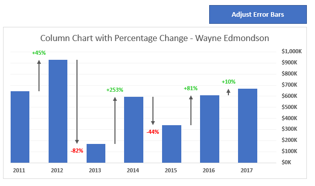
Column Chart That Displays Percentage Change or Variance - Excel Campus

Stacked bar charts showing percentages (excel) - Microsoft Community What you have to do is - select the data range of your raw data and plot the stacked Column Chart and then add data labels. When you add data labels, Excel will add the numbers as data labels. You then have to manually change each label and set a link to the respective % cell in the percentage data range.

Advanced Graphs Using Excel : create line plot with error bar plot in excel

How to Show Percentages in Stacked Bar and Column Charts - Excel Tactics To add percentage labels to the stacked column chart, first select the chart. In the new XY Chart Labels menu tab, click Add Labels. In the Add Labels dialog box that appears, choose the Data Series you would like to label (in the example, you can start with North ). Click on the field under Select a Label Range.

How to Add Data Labels to your Excel Chart in Excel 2013 - YouTube

How to add percentage labels to top of bar charts? -Put a label "Year" in your source data -Select all your data -Create the chart bar/line chart -Then select the line part of the chart and right-click -Choose show data labels - then delete the line -finally place the % labels where you want them to be...

Tableau Bar Chart Labels Overlapping - Free Table Bar Chart

Data Bars in Excel (Examples) | How to Add Data Bars in Excel? - EDUCBA Data Bars in Excel is the combination of Data and Bar Chart inside the cell, which shows the percentage of selected data or where the selected value rests on the bars inside the cell. Data bar can be accessed from the Home menu ribbon's Conditional formatting option' drop-down list.

Share :